Start R Kit: From Nothing to Data Visualization

So you want to learn R

Lots of people do, I’m starting to learn it myself. While doing so here is a quick start guide to visualizing data in an Ubuntu environment. Macs and Windows have a similar set up.

First you must install R itself found here -> https://cran.r-project.org/ 

And the main IDE for R, R Studio found here Download https://rstudio.com/products/rstudio/download/ and install for your operating system, I installed ubuntu 18.

Then open up a console and run these commands to install the system packages needed for certain R packages (for ubuntu, not other opperating systems)

• sudo apt-get install r-base-dev
• sudo apt-get install -y r-cran-httr
• sudo apt-get install libxml2-dev libssl-dev libcurl4-openssl-dev

Now we are able to open R Studio by going to Applications in the bottom left of the screen. In the R Console in the bottom left pane of the R Studio UI run this command:

• install.packages(c(“tidyverse”,”dslabs”))

Then create your first R script file, press Crtl-shift-N and save the file as whatever you please.

 

Next place the following code, here we get a data frame containing information about the number of murders per state in the United States.

"""

library(tidyverse)

library(dslabs)

data(murders)

 

murders %>%

 

ggplot(aes(population, total, label=abb, color=region)) + geom_label()

"""

Now to see the plot of data, hit the “Source with Echo” which is located in the bar above the script you just wrote.

So lets see what we get… and...

 

BAM! it should look like this.

Now lets breakdown whats going on here:

 

Importing libraries:

library(tidyverse)

library(dslabs)

# happens at top of file, is used to import modules/data/added functions

 

Creating date frame:

data(murders)

#here we create a data frame called murders from the dslabs library

 

Looking at data frame:

head(murders)

# to get a sense of the data being examined, look at the data frame and note the    columns, you should see first ten lines starting with alabama

RESULTS:

state abb region population total 

1    Alabama  AL  South    4779736 135

…

 

Murders data has to be then “piped” into the ggplot() function:

 

murders %>%

ggplot(aes(population, total, label=abb, color=region)) + geom_label()

# the data goes into the ggplot() function which is imported from tidyverse, documentation here: https://ggplot2.tidyverse.org/ 

# we feed the arguments of ggplot() with columns/categories of data from our murder data frame, labeling with the state’s abbreviation, comparing the population data (x-axis), to the total murders data (y-axis),color coating the cells based on region, and adding labels with geom_label()

 

Understanding the data:

 

Now from the graphic that was just made, we get a good sense of the most dangerous place in the United States, which says California because... well it has the most murders.

 

Unfortunately just because Cali has the most murders, doesn’t make it the most dangerous, because Cali also has the highest population, making sense of why there are so many murders there (more people=more murders)

 

What is needed is a murder rate, the number of murders based on the population, basically murders per 100,000 people.

 

Now we do not have this data, but we can create it. Let’s do it with a R function so we learn how to implement a simple one.

 

To create a function, we have to assign it to a variable, similar to creating a simple vector

 

 x <- c(1,2,3,44)

# giving the variable x a list of four numbers by using the c(), concat function

 

ratefunction <- function(tot,pop){

tot/pop*100000

}

#this function takes in two arguments, and returns the murder rate per 100,000

 

Now we want to use this function to create a new column in the murders data frame, so we can get the murder rate for each state.

 

In R, the mutate() function is exactly what we want, which modifies the existing data frame by adding a custom column of data.

Let mutate murders to include the rate.

 

ratefunction <- function(tot,pop){

  tot/pop*100000

}

murders <- mutate(murders,rate=ratefunction(murders$total,murders$population))

 

Now lets simple replace total murders in our original plot with murder rate to see the difference:

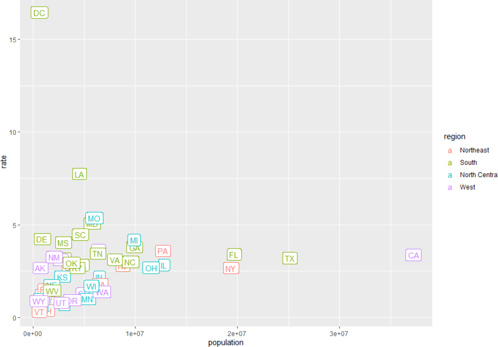
This is a more accurate showing of what states are the most dangerous based on their height on the y-axis, and get a sense of how big the state is by its population.

 

Now if we wanted to see the results by region(north/south/east/west), instead of population, we can change the ggplot() population to region like this:

 

murders %>%

  ggplot(aes(region, rate, label=abb, color=region)) +

  geom_label()

Now we see the regions with highest rates and how each state in region contributes to the murder rate.

 

Another easier and quicker way to see this is with a box plot for the regions,

Where we are comparing the rates to the regions:

 

boxplot(rate~region,data=murders)

 

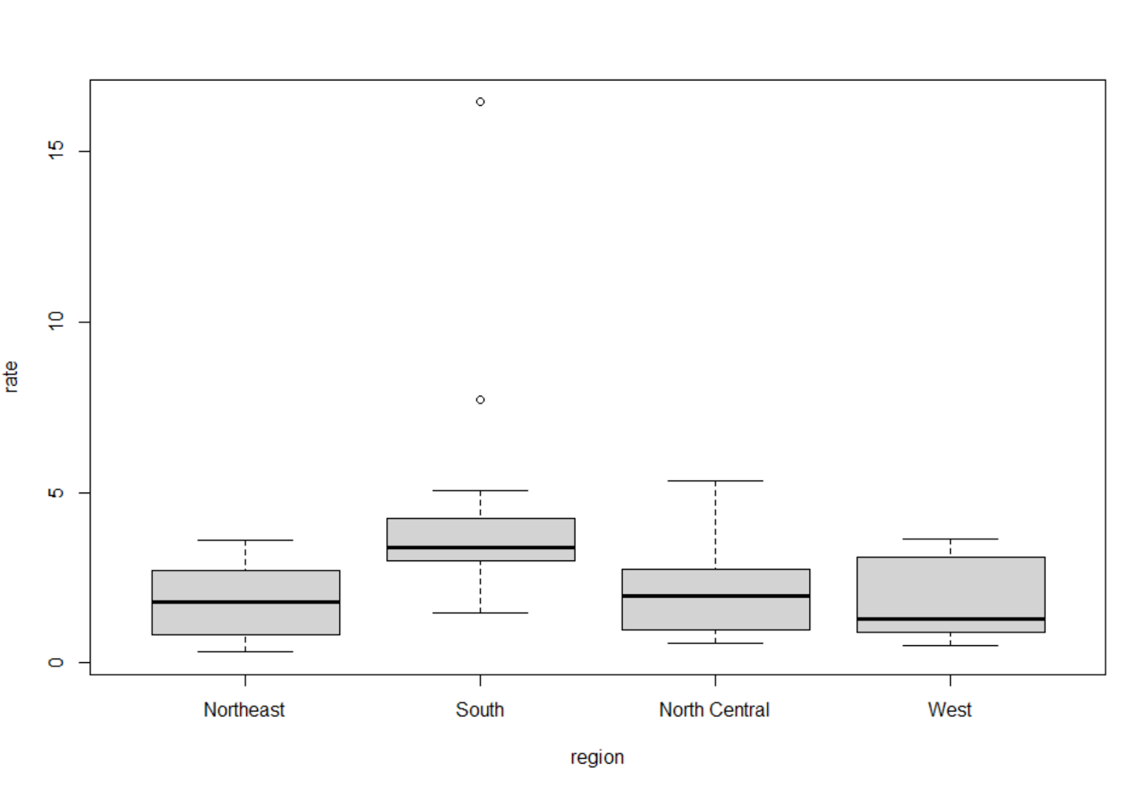
And you can notice the outliers in the box plot graph can be identified in the graph before the box plot.

 

Okay, now that we see and get a sense of the data. Now lets sort it based on wanting to see the order of the states with highest murder rates.

 

First we need to create an index variable that has the ascending order (lowest murder rate to highest), and set that to ind

 

ind <- order(murders$rate)

 

Second we access the data wanted in murders data frame = $state aka the state’s name, and we want it ordered by the index order above (ind), however because order gives us ascending, we wrap rev(), the reverse function around ind, so we get the states with the highest murders rates first.

murders$state[rev(ind)]

 

And here is our list:

> murders$state[rev(ind)]

 [1] "District of Columbia" "Louisiana"            "Missouri"            

 [4] "Maryland"             "South Carolina"       "Delaware"            

 [7] "Michigan"             "Mississippi"          "Georgia"             

[10] "Arizona"              "Pennsylvania"         "Tennessee"           

[13] "Florida"              "California"           "New Mexico"          

[16] "Texas"                "Arkansas"             "Virginia"            

[19] "Nevada"               "North Carolina"       "Oklahoma"            

[22] "Illinois"             "Alabama"              "New Jersey"          

[25] "Connecticut"          "Ohio"                 "Alaska"              

[28] "Kentucky"             "New York"             "Kansas"              

[31] "Indiana"              "Massachusetts"        "Nebraska"            

[34] "Wisconsin"            "Rhode Island"         "West Virginia"       

[37] "Washington"           "Colorado"             "Montana"             

[40] "Minnesota"            "South Dakota"         "Oregon"              

[43] "Wyoming"              "Maine"                "Utah"                

[46] "Idaho"                "Iowa"                 "North Dakota"        

[49] "Hawaii"               "New Hampshire"        "Vermont" 

 

And those are some R basics, enough to get you playing with visualizations while grouping and sorting the data.

 

Data visualization in R. Easy. Breezy. Beautiful. WondRful.

 

Take it easy.

 

- Dom

June 15, 2020, 6 a.m.